Simple Moving Average (SMA) Indicator

Exploring the Simple Moving Average (SMA) Indicator Using the Python TA-Lib Library
Disclaimer: This blog post is for educational purposes only and does not constitute financial advice. Trading involves risk, and it’s essential to perform thorough research and consult with a financial advisor before making trading decisions.
Exploring the Simple Moving Average indicator using the TA-Lib python library. This blog forms part of an ongoing series, Technical Analysis in Python, where I look into key trading indicators and their practical applications.
The Simple Moving Average (SMA) is a widely used metric that calculates the average price of an asset, typically its closing price, over a specified number of days.
In this blog, I will demonstrate how to compute and utilise SMA with Python’s TA-Lib library, providing valuable insights for algorithmic trading strategies.
Definition & Key Points
The Simple Moving Average (SMA) calculates the average of a selected range of prices, typically closing prices, by the number of periods in that range.
It is called “moving” because it continuously updates as new data becomes available and old data drops off.
Here are the key points for the Simple Moving Average (SMA) trade indicator:
- Average Price: SMA calculates the average price of an asset over a specified number of periods.
- Trend Smoothing: It smooths out price fluctuations to reveal underlying trends more clearly.
- Lagging Indicator: SMA is a lagging indicator, meaning it reflects past trends rather than predicting future ones.
- Key Levels: Helps identify support and resistance levels, trend direction, and potential reversal points.
- Trend Signals: Price above SMA may indicate an uptrend, while price below may suggest a downtrend.
- Common Periods: Commonly used periods include 10, 21, 50, and 200 days.
SMA Calculation
Calculating the Simple Moving Average is straightforward. It involves summing up the closing prices of a specified number of periods and then dividing by the number of periods. \[SMA_t = \frac{P_1 + P_2 + P_3 + \dots + P_N}{N}\]
Where:
- \(P_1, P_2, \dots, P_N\) are the prices or values over \(N\) periods.
- \(N\) is the total number of periods.
Python Example Using TA-Lib
Now, let’s implement the Simple Moving Average using Python’s TA-Lib library. TA-Lib is a popular technical analysis library that provides a wide range of indicators, including SMA. If you haven’t installed TA-Lib yet, you can do so using pip. Note that TA-Lib requires the underlying C library to be installed on your system.
Basic Example: Time period
This example calculates the Simple Moving Averages (SMA) of a predefined array of prices for three different time periods: 5, 7, and 9 days.
import talib
import numpy as np

# Example prices
prices = np.array([10, 11, 12, 13, 14, 15, 16, 17, 18, 19], dtype=np.float64)

# Calculate SMA with different timeperiods
sma_5 = talib.SMA(prices, timeperiod=5)
sma_7 = talib.SMA(prices, timeperiod=7)
sma_9 = talib.SMA(prices, timeperiod=9)

# Print the calculated SMA
print("5-period SMA:", sma_5)
print("7-period SMA:", sma_7)
print("9-period SMA:", sma_9)
After calculating the SMAs, it prints the resulting values, which display nan for the initial periods where there isn’t enough data to perform the average calculation.
5-period SMA: [nan nan nan nan 12. 13. 14. 15. 16. 17.]
7-period SMA: [nan nan nan nan nan nan 13. 14. 15. 16.]
9-period SMA: [nan nan nan nan nan nan nan nan 14. 15.]
Basic Example: Price
This example leverages TA-Lib’s abstract interface to compute the 3-period Simple Moving Average (SMA) for both the ‘open’ and ‘high’ price data provided in the inputs dictionary.
import numpy as np
from talib.abstract import SMA

# Example prices
inputs = {
    'open': np.array([2, 3, 4, 5, 6, 7], dtype=np.float64),
    'high': np.array([4, 5, 6, 7, 8, 9], dtype=np.float64),
    'low': np.array([1, 2, 3, 4, 5, 6], dtype=np.float64),
    'close': np.array([3, 4, 5, 6, 7, 8], dtype=np.float64),
    'volume': np.array([5, 5, 5, 5, 5, 5], dtype=np.float64)
}

# Calculate SMA based on different prices
sma_open = SMA(inputs, timeperiod=3, price='open')
sma_high = SMA(inputs, timeperiod=3, price='high')

# Print the calculated SMA
print("SMA Price(Open):", np.round(sma_open, 1))
print("SMA Price(High):", np.round(sma_high, 1))
After performing the calculations, it prints the resulting SMA values for the specified price types.
SMA Price(Open): [nan nan  3.  4.  5.  6.]
SMA Price(High): [nan nan  5.  6.  7.  8.]
Example: SMA BTC:USD
This example retrieves the last five days of hourly Bitcoin (BTC-USD) price data from Yahoo Finance using the yfinance library.
It then computes a 10-period Simple Moving Average (SMA) of the closing prices with the help of the TA-Lib library and appends this SMA as a new column to the dataset.
import plotly.graph_objects as go
import talib
import yfinance as yf

ticker = 'BTC-USD'
period = '5d'
interval = '1h'
sma_period = 10

# Fetch historical stock data from Yahoo Finance.
data = yf.download(ticker, period=period, interval=interval)

# Calculates the Simple Moving Average (SMA) using TA-Lib.
sma = talib.SMA(data['Close'], timeperiod=10)
data[f'SMA_{sma_period}'] = sma

data.tail(10)
The code displays the last ten rows of the updated data, which now include the calculated SMA values.

Data Output.
The next set of code removes any rows from the data DataFrame that contain NaN values in the SMA column to ensure that the dataset is complete for plotting.
# Drop rows with NaN values in SMA
data.dropna(inplace=True)

fig = go.Figure()

fig.add_trace(go.Scatter(x=data.index, y=data['Close'], mode='lines', name='Closing Prices', line=dict(color='blue')))
fig.add_trace(go.Scatter(x=data.index, y=data[f'SMA_{sma_period}'], mode='lines', name=f'SMA {sma_period}', line=dict(color='red')))
fig.update_layout(title=f'{ticker} Closing Prices and {sma_period}-Day SMA', xaxis_title='Date', yaxis_title='Price ($)', legend=dict(x=0, y=1), hovermode='x unified')

fig.show()
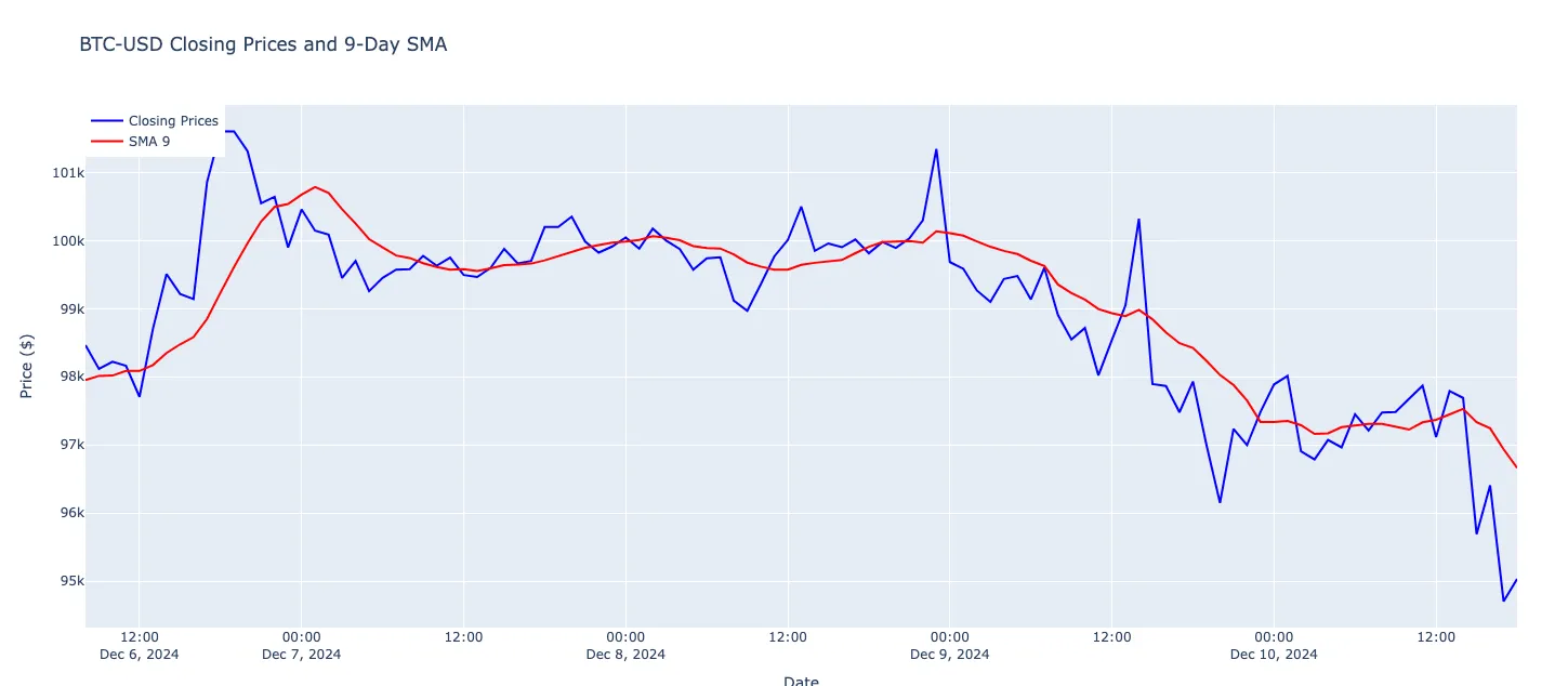
It then creates an interactive Plotly figure that overlays the closing prices and the specified Simple Moving Average (SMA) as blue and red lines respectively, sets appropriate titles and labels for the axes, and displays the resulting chart.

SMA Graph
The generated diagram illustrates Bitcoin’s closing prices over time as a blue line, with a 9-period Simple Moving Average (SMA) depicted as a red line smoothing out the price fluctuations.
When the closing prices rise above the SMA, it may indicate upward momentum and potential buying opportunities, whereas prices dropping below the SMA can suggest downward momentum and possible selling signals.
This can help traders to identify trends and reversals based on the interplay between the price and the SMA.
Conclusion
The Simple Moving Average is a fundamental tool in the arsenal of traders and algorithmic trading systems. Its simplicity and effectiveness in trend identification make it an excellent starting point for building more complex trading strategies.
By leveraging Python and libraries like TA-Lib, you can seamlessly integrate SMA calculations into your trading bots, enabling automated and data-driven decision-making.
In the next posts of this series, we’ll explore additional indicators, delve deeper into algorithmic trading strategies, and demonstrate how to combine multiple indicators to enhance your trading bots’ performance. Stay tuned and happy trading!
